The normal distribution

The normal distribution, also called the Gaussian curve or bell curve, is one of the most important concepts in statistics. Many measurements in nature and in processes follow this bell shape. If you know a process is normally distributed, you can predict its performance well from a limited number of measurements. That is why the normal distribution plays a big role in Six Sigma.

What is the normal distribution?

The normal distribution is a symmetrical probability distribution with one peak in the middle and ever smaller probabilities towards both sides. Two numbers define the whole distribution:

• The mean (μ, mu): the centre of the curve, the typical value.
• The standard deviation (σ, sigma): the width of the curve, or how far measurements lie around the mean on average. Strictly speaking, it is the square root of the average squared distance from the mean.

The 68-95-99.7 rule

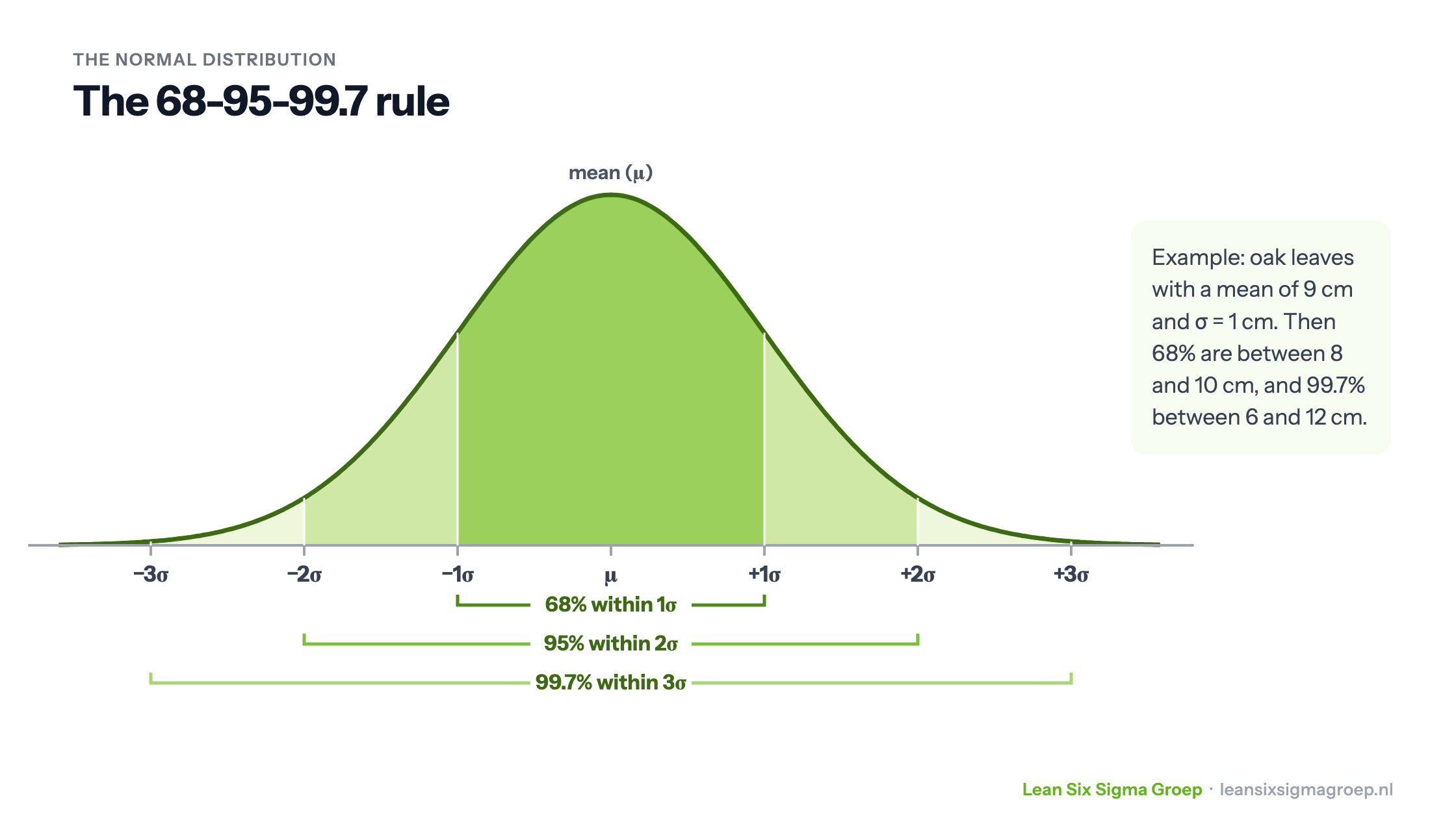
An important property is the empirical rule, shown in the image at the top of this article:

• about 68% of measurements lie within one standard deviation of the mean;
• about 95% within two standard deviations;
• about 99.7% within three standard deviations.

An example: if you measure the leaves of an oak tree, with a mean length of 9 cm and a standard deviation of 1 cm, then 68% of the leaves are between 8 and 10 cm long, and 99.7% between 6 and 12 cm. A leaf of 13 cm is so exceptional that it is worth investigating.

How does a normal distribution arise?

A normal distribution often arises when a measurement is the result of many small, independent, random influences. That is why it is common in nature, in lengths, weights and measurement errors.

Not everything is normally distributed. Lead times, for example, are often skewed: they can’t go below zero, but they can run very long. A special cause, such as a machine going out of adjustment, also disturbs the normal distribution. So always check first whether your data is normally distributed, for example with a histogram or a normality test, before you calculate with it.

The central limit theorem explains why the normal distribution is still so often useful: if you repeatedly take a sample and calculate its mean, those means are approximately normally distributed, even if the individual measurements are not. This applies to means, not to individual measurements.

The normal distribution in Six Sigma

Six Sigma aims to improve process quality by reducing variation. The normal distribution helps describe how a process behaves. If the data shows a process is normally distributed, and around 30 measurements is often enough for that, you can calculate further with it.

Z-score and sigma level

The Z-score links the customer requirement to the process. It shows how many standard deviations fit between the process mean and the limit set by the customer. From the Z-score follows the probability of a defect: the part of the curve beyond the limit.

The Z-score is also called the sigma level, which is where the name Six Sigma comes from. A process at Six Sigma level produces, with the usual 1.5 sigma correction for long-term shift, 3.4 defects per million opportunities.

Defects per million opportunities (DPMO)

DPMO is the number of defects per million opportunities for an error. You simply count it, but with the normal distribution you can also calculate it in advance from the mean and standard deviation, and convert it into a sigma level. That makes the performance of different processes comparable. Also read about Cp and Cpk, which express process capability in the same way.

Control charts

A control chart shows the results of a process over time, with the mean and an upper and lower limit at three standard deviations: the Upper Control Limit (UCL) and the Lower Control Limit (LCL). In a stable process, 99.7% of the points fall within these limits.

Points within the limits belong to the normal variation of the process, common cause variation. A point outside the limits, or a striking pattern such as seven points in a row on one side of the mean, points to a special cause, special cause variation. You investigate that. The smaller the standard deviation, the closer together the limits are.

DMAIC

In the Measure and Analyse phases of DMAIC, you use the normal distribution to describe data, determine process performance and test differences.

Practical example: filling bottles

A machine fills 500 ml bottles. A bottle may not contain less than 490 ml. The team measures that the fill is 500 ml on average, with a standard deviation of 5 ml.

In the Black Belt training you go into this in more depth, with statistical analysis.

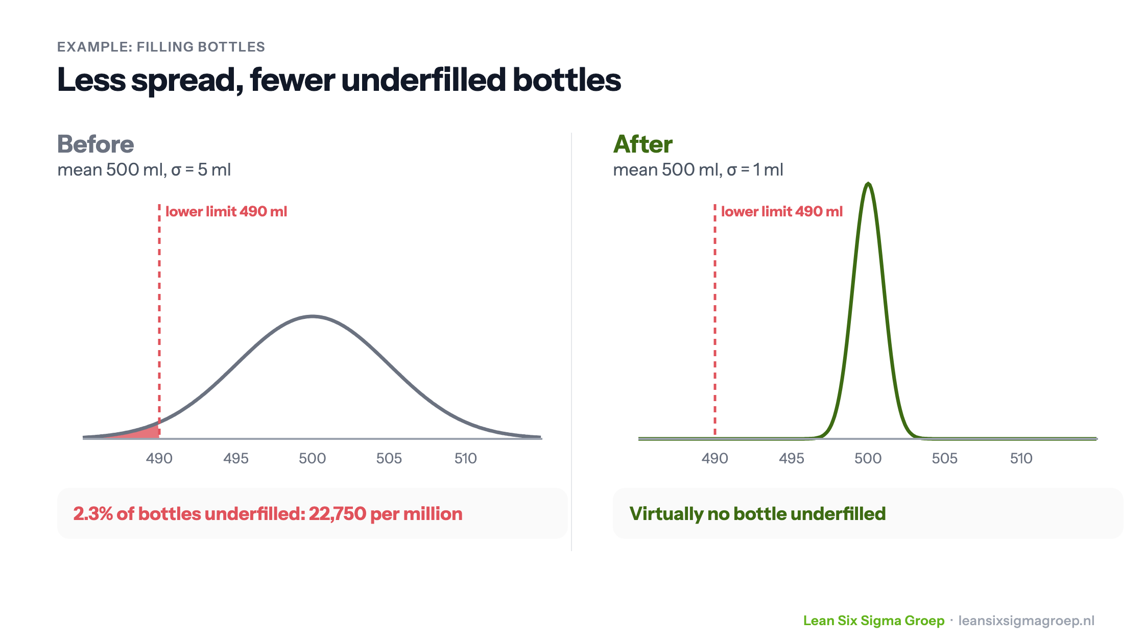
The lower limit is then two standard deviations below the mean (Z = 2). According to the normal distribution, 2.3% of bottles fall below it: 22,750 per million. Using DMAIC, the team finds the causes of the variation, calibrates the filling machine and trains the operators. The standard deviation drops to 1 ml. The lower limit is now ten standard deviations from the mean, and virtually no bottle is underfilled any more. The mean hasn’t changed: only the variation has become smaller.

Conclusion

The normal distribution helps you understand variation and decide, based on data, how to improve a process. Less variation means fewer defects, more efficient processes and more satisfied customers.

The video with this article gives a short explanation of the normal distribution and its properties.

Want to learn to work with the normal distribution, statistical analysis and control charts yourself? That is covered in depth in the Green Belt training course.