Mode

The mode is the value that occurs most often in a dataset. It is one of the three measures of central tendency, alongside the mean and the median. For categories, such as types of complaints or reports, the mode is even the only measure of central tendency you can use.

The mode in everyday life

I commute to the office every day and by now know how long I spend travelling on average. When I order firewood, I know how much I use in an average winter. These are all measures of central tendency: one number that says what “normal” is.

The mode seems less familiar, but you come across it more often than you think. Take modal income. In the Netherlands, the Central Planning Bureau works with modal income, the income most common among employees; the typical Dutch person is even nicknamed “Jan Modaal”. Average income is higher: a relatively small group with high incomes pulls the mean up. For the question of what a policy means for most people, the mode is therefore a better yardstick than the mean.

Mode, median and mean

• Mode: the value that occurs most often.
• Median: the middle value when all values are put in order.
• Mean: the sum of all values, divided by the count.

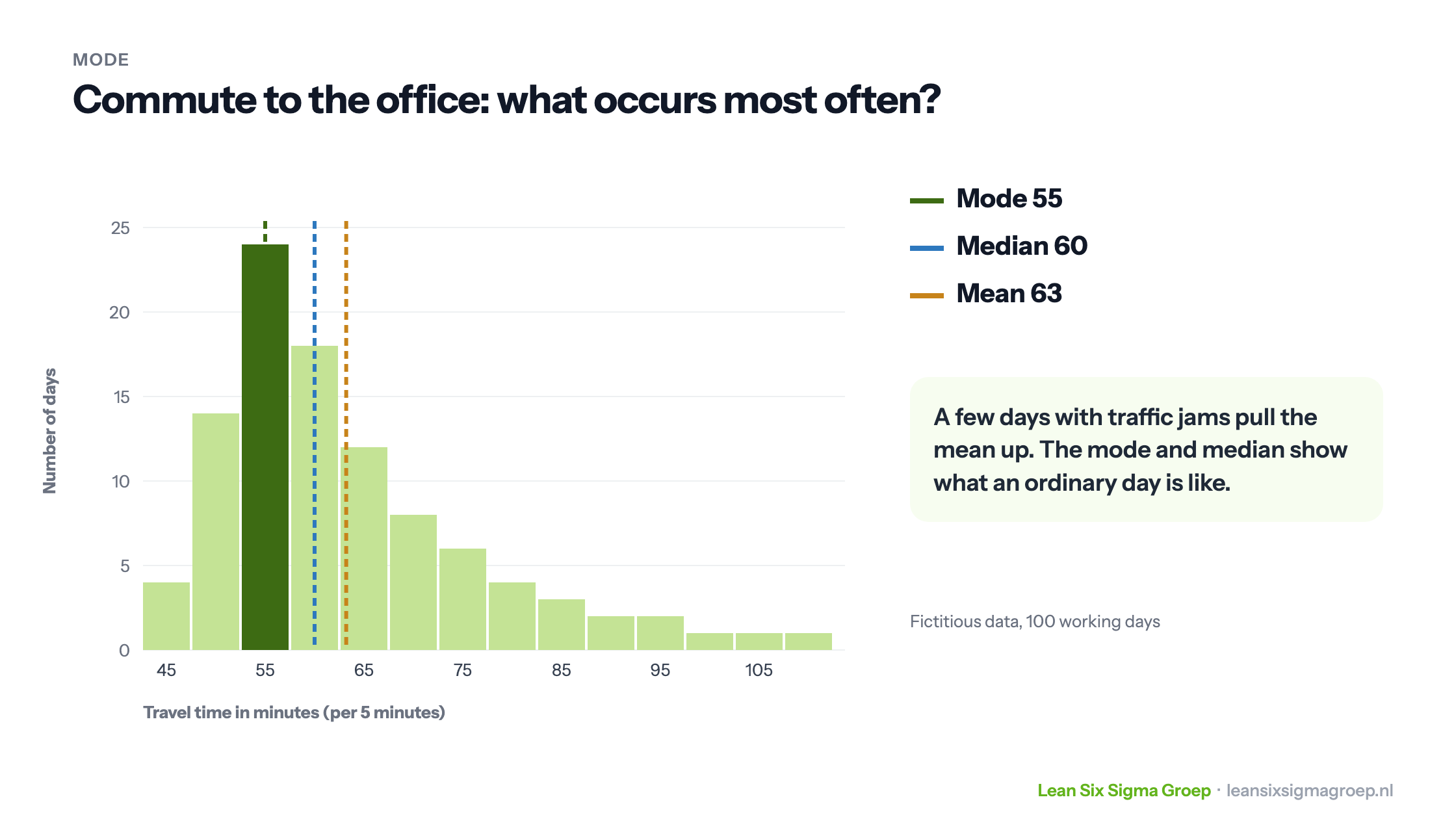
With a symmetrical distribution, such as the normal distribution, they lie close together. With a skewed distribution they don’t. The image at the top of this article shows an office worker’s travel time in a histogram, rounded to five minutes. On most days the journey takes 55 minutes: that is the mode. The median is 60 minutes, the mean 63. A few days with traffic jams pull the mean up, while the mode shows what an ordinary day is like.

Mode for continuous data

With continuous data, such as time or weight, each exact value often occurs only once. A temperature with two decimals has no real mode. That is why you first group the data into classes, such as travel time per five minutes. The class with the most observations is the modal class, and its midpoint counts as the mode.

Mode for categories

For data consisting of categories, such as types of reports, car brands or satisfaction scores, a mean has no meaning. What is the average report? You can determine the mode, as shown below.

This is one of the tools you learn to apply in the Green Belt training.

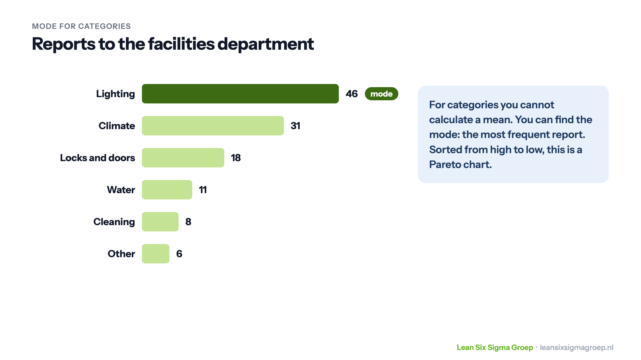
A facilities department receives reports from across the organisation and sorts them by type: the lighting doesn’t work, it is too warm, a door doesn’t close. The most frequent report, lighting, is the mode, and perhaps deserves attention first.

More than one mode

If two or more values occur equally often, the dataset has several modes: bimodal with two, multimodal with more. A distribution with two clear peaks is often a sign that two groups are mixed together: for example travel time on days by car and days by train, or the lead time of two teams that work differently. That is a hint to split the data and look at each part separately.

The mode and Pareto

In Lean Six Sigma you often meet the mode in a Pareto analysis. There you rank categories by how often they occur, from high to low. The first bar is the mode. Often a small share of the categories turns out to cause most of the problems: the well-known 80-20 rule.

Examples

• Services: the most frequent complaint, such as long waiting times, indicates which improvement project deserves attention first.
• Government: the most reported problem in a neighbourhood shows where policy makes the biggest difference.
• Financial services: the most common type of transaction determines which process must run smoothly first.
• Manufacturing: the most common type of defect is often the best place to start.

The video below shows how to apply the mode and the other measures of central tendency.